White Dwarf Pulsations Are Like An LRC Circuit

Lately, I’ve been struggling to wrap my head around the driving of pulsations in DAV white dwarfs. The canonical set of papers on this topic are the series by Yanqin Wu and Peter Goldreich, starting with this one which is mostly the one I’ll stick to today.

They consider high-frequency white dwarf g-modes, for which we can basically split the star into four regions. Starting from the center of the star, the first relevant point is the point at which the angular frequency of our mode is equal to the Lamb frequency: $\omega = S_\ell$. This is the outer turning point of the g-mode cavity, and it’s at a depth from the photosphere we’ll call $z_\omega$. Travelling out of the star from this point, we move through the upper evanescent zone, where the eigenfunction with eigenvalue $\omega$ transitions from oscillatory to exponential behavior. In this region, the pulsations which propagate in the g-mode cavity are going to be radiatively damped.

The upper evanescent zone ends when we hit the base of the convection zone at depth $z_b$. We’ll assume that the mode under consideration has high enough frequency that $z_b « z_\omega$. The convection zone is very shallow in the star, so it’s safe to assume that once we’ve travelled out of the convection zone, the remaining depth to the photosphere is very small. That’s important, because presumably this will be another region of radiative damping.

Wu and Goldreich (1999) show that the stability of a mode is governed by two competing factors: the driving induced by the convection zone, and radiative damping from the upper evanescent zone. Formally, in the non-adiabatic (or quasi-adiabatic) case, an eigenvalue is a complex number which can be written as

and solutions have time dependence $\propto \exp(i\omega t) = \exp(\gamma t)\exp(i\omega_R t)$. So in regions where $\gamma > 0$, the mode will grow, and in regions where $\gamma < 0$ the mode will decay. The paper shows that the upper evanescent zone has $\gamma_\text{rad} < 0$ and so always decays, and the convection zone has $\gamma_\text{cvz} > 0$ and so the mode is driven. The net stability of the mode is given by

with $\mathcal{A}$ a nondimensional constant defined in the paper, $(\delta p/p)_b$ the pressure perturbation at the base of the cvz, and $\tau_c$ the convective timescale.

The Response of the Convection Zone to Forcing

I want to understand why the convection zone behaves this way. There’s a complex term in the driving of the mode through the convection zone. This is because the convection zone does not respond instantly to the incoming pulsation. Instead, some of the flux will be delayed as it travels through the convection zone due to the nonzero convective timescale and the heat capacity absorbing some of the energy. I think the effect of the convection zone on the flux perturbation at its base is similar to the behavior of a capacitor in an LRC circuit. Consider the following circuit:

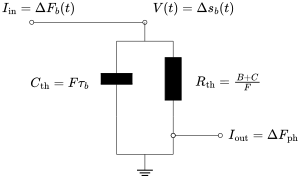
Here, $I_\text{in}$ is a stand-in for the flux at the base of the convection zone, the capacitance $C_\text{th}$ represents the thermal capacity of the convection zone, $R_\text{th}$ represents the heat which is dissipated by the convection zone, and $I_R$ is the flux perturbation which travels out of the zone and into the photosphere. The ground connection is a bit of a construct here that we can use to actually simulate the circuit, but we can think of it as representing the equilibrium entropy of the star (that is, when we set $\Delta s_b = 0$, the convection zone circuit is not driven).

The voltage of this circuit is a stand-in for the time-dependent perturbation to entropy at the base of the cvz, which the paper writes as $\Delta s_b(t)$. One thing to keep in mind is that an efficient convection zone is isentropic, and responds approximately instantly to entropy perturbations. What this means is that the entire convection zone can be characterized by a single scalar: the time-dependent perturbation $\Delta s_b(t)$ at the base. This is why this parameter is a good stand-in for voltage. We can apply Kirchoff’s rule for current to the node:

Rearranging this, and using the assumed form of the time derivative $\partial/\partial t \to -i\omega$, we can rewrite this as

The paper gives us the relationship between the flux and density perturbations at the bottom of the cvz:

where I’ve used definition (43) from the paper. This equation is useful because it lets us determine the strength of driving in the convection zone as a function of the convective timescale $\tau_c$ and the strength of the perturbation. In the circuit analogy, this represents something not unlike the voltage as a function of the input current and the capacitance.

We can also use this circuit to determine the flux perturbation which emerges from the photosphere. In the analogy, that’s going to be given by the current $I_\text{out}$. We have a current $I_\text{in}$ flowing into that node (since current is constant over the resistor). Out of that node flows the current which was otherwise lost over the capacitor and the current which flows to the photosphere:

and using the previous relation,

This is exactly the form specified in the paper. I think you could reproduce any of the relations in the paper using a careful and dimensionally consistent Kirchoff analysis of the above circuit.